Wind turbines and solar panels are energy conversion devices. The input to these systems is not constant, it changes with the seasons, the weather and the time of day.
Comment
This work has not been reviewed, thus it should be treated as a discussion not a description.
Wind
Wind is the result of uneven heating of the Earth's surface, in addition to climate, the airflow over any given location will be influenced by terrain. There can be significant variation in the wind experienced by places only a few kilometres apart. Whilst wind is often described in terms of velocity and direction of travel, it can be useful to consider it in terms of power. The wind power available for conversion by a turbine is related to the cube of its velocity.
Power = area * density * velocity3 / 2
A small increase in wind speed represents a large increase in energy, for example wind blowing at 8 m/s has more than twice the energy than at 6 m/s.
By setting the area equal to 1 square metre and approximating the density of air to 1.2 kg/m3 and converting the units to kw, the formula reduces to:
Power = 1.2 * Velocity3 / 2000
Comparisons based on this formula should be treated with caution. The density of air falls with increasing altitude, for example it is close to 1.0 around 1,500m. The height of the observation above ground also has an influence, for a few hundred metres above the surface, the wind speed increases with height above ground as the effect of friction reduces. The power of a wind turbine is substantially less the value given by this formula as only a fraction of the energy is extracted. The fraction of the energy extracted at any given time is known as the coefficient of performance, typically this is in the range 0.1 to 0.4 and may vary according to the wind speed.
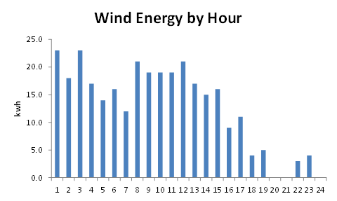
If enough data is available, then estimates of power (the rate of doing work) can be used to make an estimate of the wind energy passing over the point of observation during a given time period. The graphs below are are based on a randomly selected location and are an estimate of the wind energy by month, day and hour.
The first graph shows the cumulative wind energy broken down by month, In this example, there is significant seasonal variation, this may vary with climate. In Western Europe peaks in wind energy often cluster around the equinoxes. However, in general, there is some correlation between the periods of peak wind energy and the demand for electricity which also peaks in winter.

Breaking the same dataset down by day shows that wind energy tends to be packaged in pulses a few days apart.

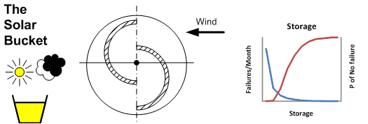
This pattern is present in many sets of observations. This pattern of supply makes it necessary to have either an element of buffer storage in the system or an alternative that provides an adequate supply of energy in during the periods of relatively low output.
Many areas have a pattern of diurnal variation, In coastal areas this can be caused by the different heating/cooling behavior of land and sea with the direction and intensity changing with night and day.
These short term fluctuations emphasise the need for storage or alternative means of generation which can respond quickly to changes in supply and demand.
Solar
The principal variation in solar irradiance comes from Sun-Earth geometry. The Earth's axis is inclined relative to its orbital plane, in the Northern hemisphere the pole is inclined towards the Sun in summer and away from it in winter and each day the Earth rotates about its own axis. As a result the solar irradiance varies during the day, and seasonal variations are related to latitude.
The graph below shows the estimated clear sky solar irradiance over the course of the day for Southern England (approx. latitude 51 deg. N) at four times of the year.

Superimposed on the variations imposed by planetary motion is the influence of atmospheric conditions, the most significant of these is the effect of clouds. Clouds are a feature of climate, itself closely related to latitude. The height and extent graphics below illustrate the variations. These diagrams are compiled from the height and extent of the cloud cover at solar noon.
The first is for a maritime temperate climate, such as the South of England.

Clouds limit the solar radiation reaching the Earth's surface through a combination of absorption and reflectance. In general, low, thick overcast cloud such as stratus can attenuate irradiance by more than 80%, whilst the effects of high level cloud such as cirrus may only cause 20% attenuation. In southern England winters are characterized by periods of low and very low overcast skies. In summer the general pattern consists of few, scattered or broken cumulus, the attenuating effect of these summer clouds is less than those of winter and the overall effect is to cause fluctuations in the output of solar devices.
A significantly different climate to that of Southern England is that of Arizona, whose height and extent diagram is shown below.

The principal difference is the much lower frequency of occurrence of low level cloud and less seasonal variation.
The effects of planetary motion and cloud cover are combined in the simulation of solar irradiance over Southern England which is shown below:

This graph is based the solar radiation received by a horizontal surface, such as a field. In most cases the yield of solar devices is increased by tilting them towards the Sun. Output can be further enhanced by mounting the panels on a tracking device which ensures the panels are always pointing directly at the Sun, however the extra yield must be set against the cost of the the tracking mechanism.
The graph below shows the effect of cloud on the output of a solar device. It was compiled from three sets of observations taken around solar noon in June 2011 each with a different cloud extent.

Description of Diagrams
The core of both sets of diagrams is a database of weather and related reports.
- Cloudbase and Extent - The diagrams are an attempt to show variation in the nature of cloud cover with climate. The diameter of the circle indicates the frequency of occurrence and those representing cloud cover are pie charts showing the proportion of the extent. Extent is described using the descriptions used in Metar reports, e.g.FEW (1 - 2 Octas), SCaTtered (3 - 4 Octas), BroKeN (5-7 Octas) and OVerCast (8 Octas). Cloud is described as high, if the base is greater than 18,000 feet, low if less than 6,000 feed and very low if it is less than 1,000 feet. Only the highest, most significant layer is used in the computations. It is planned to evolve these diagrams to include more layers, the code was originally intended for use with Western Europe data where the lowest layer is frequently the most significant, however, they do not provide a full picture of the sky in monsoon areas where the sky can be significantly more complex.
- Wind - The wind related graphs are based on SQL retrievals from a database of weather reports which were clipboarded into Excel. Datasets where chosen which had an almost complete set of hourly observations for a given year. There are some anomalies in the process, but it is thought that the results give are reasonable description of the variation in wind speed over time.

No comments:
Post a Comment