But its also having fun with a kite.
The kite was given to me as a Christmas present by my son (aged 23 at the time, him not me). It's a small kite which fits easily into a pocket and would be ideal for business people. One can imagine herding the participants of a meeting into the car park and sending the kite aloft. Then point upwards and exclaim "that's were we should be", followed by a profound silence and the sensible one saying "shall we go back inside now?".
Despite a complete lack of electronics and telemetry, the kite gives an insight into the the nature of wind at heights between 5 and 25 metres (maybe higher, I replaced the original string with a longer one and its still climbing). Last Saturday when the wind was blowing 3 - 4 m/s, I took the kite to two different locations. The first was a beach where the wind was coming in off the sea and the second was a public park in an urban area a mile or so north of the seafront. The behaviour of the kite was significantly different at each site.
On the beach, the kite effortlessly took to the air and was stable at a height of 5m and the trailing streamers had no difficulty in keeping it head up to the wind. Once the string was fully unwound, the kite sat comfortably in the sky, maybe with the odd flutter, but I was able to hook the handle on to the bike and take the photo at the top of the page. After half an hour, I felt guilty about bringing it back to Earth.
At the park, things were different. I almost pointed out to the man mowing the cricket pitch who cast disapproving looks in my direction, that what he was going to do on the grass later in the day was no less ridiculous than what I was doing but life's too short for pointless conversations. Here the kite struggled with turbulence up to, say, 15m and getting it airborne required many attempts, hoping that it would acquire enough upward motion to counter any downward influences. With patience, it was possible to get the string fully extended, but the kite was never stable and was prone to twisting and each twist tied a small knot in the string. I suggest that the number of knots in a kite string is a measure of wind turbulence. Nor did the kite stay aloft. Typically in urban areas, wind is not a smooth stream of air, but a series of gusts, often with significant gaps between then, it was in these gaps that the kite spiralled to the ground. The kite suggested that conditions measured at 2m, extend upwards to at least 25m. It was also clear that wind speed increased with height, even though the turbulence persisted.
When the next opportunity presents itself, I will take the kite into the hills to the north of the town, just because its fun.
PS - 18-Apr-2014 - I found myself on the same beach yesterday, this time the wind was coming from the NE and was blowing from the land to the sea. The turbulence that is observable inland made it hard to get the kite airborne and once aloft, it started to drift earthwards as soon as a gust had subsided.
Friday, 14 March 2014
Friday, 7 March 2014
The Rayleigh Distribution
One of the reasons for modelling a system is to get an understanding of how it might work before you build it, the logic being that paper are spreadsheets are cheap whilst metal and earth moving are expensive. There are many ways of doing this, one is to use historic data as the input, for example a time series of wind speed measurements, another is use some form maths/stats function to mimic the real world. Each approach has its strengths and weaknesses.
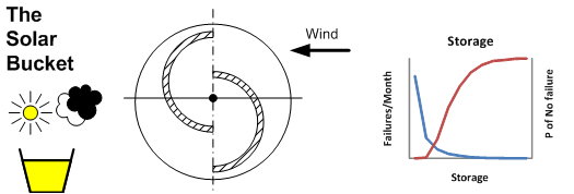
I'm currently messing with a storage based project, some initial work was done on a computer, but to make it a bit more fun, I'm building a very small prototype which is controlled by weather reports from the internet. This provides some insights which a purely maths and stats approach would hide, not the least of these is the economics of the process. In a mathematical model, changing a parameter is often just a matter of editing a line of code, with a physical model, changing something usually involves a cycle ride and spending money. This has forced some decisions on how much information is needed to drive the system and what is nice-to-have which leads to a discussion on the merits of a big budget which allows flexibility and experimentation or a small budget in which constraints may foster creativity. Such is life at the cutting edge of R and D.
As with anything on this blog, this is unreviewed work in progress which should be treated with caution.
When I first became interested in sustainable energy systems, I found a source of data which provided the average wind speed for a given location. the figure for my backyard was 5.0 m/s (I think), this might be the case for level ground devoid of trees and houses, but it was a start. To make an estimate of the energy that might be extracted from a stream of moving air, it is necessary have a distribution of the wind speed. One solution is to use the Rayleigh distribution, which with the help of spreadsheet can take an average wind speed and turn it into a histogram which is an estimate of the of the number of hours per year a given wind speed will occur. The Rayleigh distribution is a special case of the Weibull in which the shape factor is fixed at 2.0 which simplifies the process. Both the Rayleigh and Weibull distributions can be used to model wind speed. The relationship between the maths and the wind is empirical which simply means "it works" without a providing a causal mechanism. This sort of model is common in science, the goals scored in a football match can follow a Poison distribution, rainfall can follow a Gamma distribution, extremes can be described with the Pareto and Gumbel distributions (amongst others).
The graph below shows the distribution of wind speed which is estimated by the Rayleigh model and observed wind speed for a selected location with an average wind speed of 5 ms/s:
In this case, there is reasonable agreement between the estimated and observed values, in part because the dataset was chosen for this reason.
As part of a project to learn about the nature of wind as an energy source, I collected data from diverse location, which I'm still studying. The inference from this, so far, is that the Rayleigh distribution describes the wind speed distribution at an "ideal" location. It provides a reasonable model where the terrain is flat or a plateau and also for offshore wind in locations poleward of the tropics and for upper air soundings at the 850 mb level. It does not provice a good model where the terrain is complex or for urban areas. In these cases, a better solution might be to use a Weibull distribution where the shape factor is in the range 1.2 to 1.8. In these cases, the Rayleigh distribution will over estimate the energy yield.
This is a link to a more detailed description of the Rayleigh Distribution, it will be updated over the next few weeks as other work is completed.
Rayleigh Distribution
I'm currently messing with a storage based project, some initial work was done on a computer, but to make it a bit more fun, I'm building a very small prototype which is controlled by weather reports from the internet. This provides some insights which a purely maths and stats approach would hide, not the least of these is the economics of the process. In a mathematical model, changing a parameter is often just a matter of editing a line of code, with a physical model, changing something usually involves a cycle ride and spending money. This has forced some decisions on how much information is needed to drive the system and what is nice-to-have which leads to a discussion on the merits of a big budget which allows flexibility and experimentation or a small budget in which constraints may foster creativity. Such is life at the cutting edge of R and D.
As with anything on this blog, this is unreviewed work in progress which should be treated with caution.
When I first became interested in sustainable energy systems, I found a source of data which provided the average wind speed for a given location. the figure for my backyard was 5.0 m/s (I think), this might be the case for level ground devoid of trees and houses, but it was a start. To make an estimate of the energy that might be extracted from a stream of moving air, it is necessary have a distribution of the wind speed. One solution is to use the Rayleigh distribution, which with the help of spreadsheet can take an average wind speed and turn it into a histogram which is an estimate of the of the number of hours per year a given wind speed will occur. The Rayleigh distribution is a special case of the Weibull in which the shape factor is fixed at 2.0 which simplifies the process. Both the Rayleigh and Weibull distributions can be used to model wind speed. The relationship between the maths and the wind is empirical which simply means "it works" without a providing a causal mechanism. This sort of model is common in science, the goals scored in a football match can follow a Poison distribution, rainfall can follow a Gamma distribution, extremes can be described with the Pareto and Gumbel distributions (amongst others).
The graph below shows the distribution of wind speed which is estimated by the Rayleigh model and observed wind speed for a selected location with an average wind speed of 5 ms/s:
In this case, there is reasonable agreement between the estimated and observed values, in part because the dataset was chosen for this reason.
As part of a project to learn about the nature of wind as an energy source, I collected data from diverse location, which I'm still studying. The inference from this, so far, is that the Rayleigh distribution describes the wind speed distribution at an "ideal" location. It provides a reasonable model where the terrain is flat or a plateau and also for offshore wind in locations poleward of the tropics and for upper air soundings at the 850 mb level. It does not provice a good model where the terrain is complex or for urban areas. In these cases, a better solution might be to use a Weibull distribution where the shape factor is in the range 1.2 to 1.8. In these cases, the Rayleigh distribution will over estimate the energy yield.
This is a link to a more detailed description of the Rayleigh Distribution, it will be updated over the next few weeks as other work is completed.
Rayleigh Distribution
Friday, 28 February 2014
Clouds and Irradiance
Comment
This was written over a year ago to gather together thoughts and observations on the relationship between clouds and solar devices. It has not been formally reviewed, thus it should be treated with caution and as a discussion.
Solar Devices
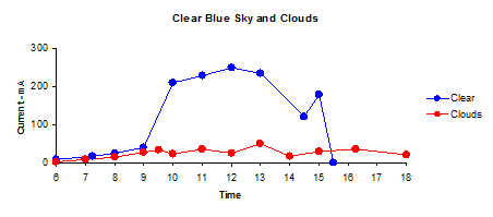
The first graph shows the current delivered to the battery between 06:00 and 18:00:
The second shows the charge supplied to the battery (in mA hours):
The "clear" and "clouds" represent the extreme cases, most days are a mix of blue sky and passing clouds.
On days when the sky state consists of a few, scattered or broken clouds there will be significant fluctuations in irradiance within a short space of time (and hence output) as can be seen in the graph below:
At the time these measurements were recorded, scattered cloud was present at an estimated height of 2 - 4,000 feet.
The Sky over Southern England
The bubble chart shows the states of the sky over southern England during a year:
The graphic does not give a full description of the sky. In summer the low cloud is typically a thin layer of cumulus which has only a moderate attenuating effect whilst in winter, the sky is overcast with a thick layer of stratus.
| Summer |
| Winter |
![]() |
| Summer |
![]() |
| Winter |
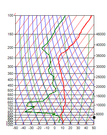
SkewT diagrams are complex, but a lot of information can be obtained visually.
When the temperature and dew point lines are far apart, the relative humidity is
low, as is the proability of cloud formation, when they are close together, the
relative humidity is high and it is probable that clouds have formed. In
the left hand diagram, the cloud is probably a thin layer of cumulus as shown in
the photo above. In winter, the high relative humidity resulting from
lower temperatures may allow can allow a thick layer of cloud to form.
Solar devices and the human body generally don't make too much
distinction between a clear blue sky and one with a few clouds in it, but a thick
overcast layer can reduce the amount of solar radiation reaching the Earth's
surface by more than 80%. This can reduce the output of solar devices and
creates a desire in the English to move closer to the Equator.
What Clouds Do
What Clouds Do
The effect of clouds is to reduce the amount of the Sun's radiant energy
transmitted to the Earth's surface. Part of the energy is reflected
upwards and part of it is absorbed within the cloud itself. This is
illustrated in the diagram below:
It shows that effect of clouds during winter is much greater than during the summer months.
Describing the effect of Clouds
There are many ways of describing the effect of clouds. Most of the comments on this site are based on the Clear Sky Factor (CSF for short), This is the ratio of the observed global horizontal iraddiance (OGH) to estimated clear sky global horizontal irradiance:
Under a clear sky, the value of CSF is constant at 1.00, under a thick, overcast sky it is usually in the range 0.1 to 0.2
The choice of GHI as a basis for a ratio is pragmatic, GHI is the most readily available form of solar irradiance data and secondly it is relatively independent of device geometry.
The second measure is the diffuse fraction which is the ratio of diffuse irradiance to total irradiance:
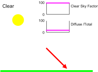
The diagrams below show how CSF and DF change with the state of
the sky. These diagrams are idealised, even a casual glance at a
clouded sky suggests that there is strong random element in the behaviour
of clouds and for this reason it might be desirable to model CSF and DF as
probability distributions.
Clear Sky
Under Pure Clear Sky conditions, there is no attenuation, the value of CSF is 1.00 and the diffuse fraction in the range 0.05 – 0.15.
Overcast Sky
At the other extreme, the modal value of CSF for a thick overcast sky is around 0.2 with a relatively narrow variation, say in the range 0.1 to 0.3. No direct sunlight reaches the ground and the diffuse fraction is constant at 1.00
The Cloudy Sky
The cloudy Sky is an intermediate state between clear and overcast. A common scenario is for cloud masses to move across the sky propelled by wind. When a sensor on the ground sees clear sky, the instantaneous value of CSF is around one and the diffuse fraction will be greater than under a clear sky. It is possible in the case of FEW clouds or high level clouds that CSF will exceed one due to the additional diffuse irradiance. When the Sun is obscured by cloud, there will be little or no direct irradiance and the diffuse fraction will approach one. Over a time interval, say 15 minutes, the time average of CSF will be proportional to the amount of cloud cover.
Precipitation and Obscuration
Rain, snow and fog are frequently associated with low, dense cloud, added to which is a layer of large droplets of liquid water. The effect, depending on the intensity of the weather is to lower the value of CSF below that expected from overcast cloud, sometimes to around 0.05.
A special case of the effects of weather on solar devices is when the receiving surface becomes covered in snow, in this case the CSF falls to zero, even though pure clear sky conditions may prevail.
The effect of Height
Cloud types are divided into three groups, low, medium and high. Low clouds are those between ground level and 6,000 feet, their formation is influenced by conditions on the ground. High clouds exist above 18,000 feet and are composed of ice crystals. It is less common for medium level clouds to exist as a single layer, they are often part of a complex sky during periods of changeable weather.
Weather reports usually only provide information on the extent of the cloud and the height of the base above ground and sometimes the type (e.g. cumulus, cirrus etc.), they do not describe the thickness. The thickness can be a function of the climate type and season, for example, the description OVC020 (overcast with the base at 2,000 feet) might describe a thin layer of stratocumulus in in a Californian summer or a thick layer of nimbostratus during a European winter. Also as the extent of the lower layer increases, less is known about the layers above, thus in the example above, there could be several layers of cloud above the overcast at 2,000 feet. The comments on are based on observations of single layers of cloud and because of the issues outlines above, should be treated as generalisations. As the complexity of the sky increases, conditions become overcast.
Low cloud has the greatest attenuating effect. Skies described as having a single layer of few, scattered or broken cloud typically have CSF values in the range 0.4 to 0.6 when the sun is obscured by cloud. The length of the period of obscuration increases as as the extent increases. As the extent becomes overcast the range of CSF values can extend from 0.6 right down to less than 0.1. The lower values being associated with thick layers of stratus or nimbostratus often with bases around 1,000 feet.
In most cases, high clouds such as cirrus have a relatively small attenuating effect ,an overcast sky of high level cloud might might have a CSF value of 0.8.
![]() |
| Add caption |
The cloud also changes the nature of the irradiance. The cloud
acts as a diffuser, when the Sun is obscured by a cloud, the irradiance is
not only attenuated, but becomes diffuse.
The proportion of energy transmitted is a function (amongst other
things) of the type of cloud, its height and thickness, the nature and
extent of the cover and the time of day. All of which conspire to
make it difficult, if not impossible to model the process.
The Seasons
Whilst the attenuating effect of clouds is a combination of reflection and absorption, there does seem to be a link between the thickness of a cloud layer and its attenuating effect. In winter, the base of low level cloud falls and the thickness increases as does the zenith angle. The graph below was inferred from data collected by the Electric Solar Bucket in the South of England.
It shows that effect of clouds during winter is much greater than during the summer months.
Describing the effect of Clouds
There are many ways of describing the effect of clouds. Most of the comments on this site are based on the Clear Sky Factor (CSF for short), This is the ratio of the observed global horizontal iraddiance (OGH) to estimated clear sky global horizontal irradiance:
Under a clear sky, the value of CSF is constant at 1.00, under a thick, overcast sky it is usually in the range 0.1 to 0.2
The choice of GHI as a basis for a ratio is pragmatic, GHI is the most readily available form of solar irradiance data and secondly it is relatively independent of device geometry.
The second measure is the diffuse fraction which is the ratio of diffuse irradiance to total irradiance:
Under a clear sky, the diffuse fraction is typically around 0.15 whilst under an
overcast sky is constant at 1.00
The effect of increasing extent
Clear Sky
Under Pure Clear Sky conditions, there is no attenuation, the value of CSF is 1.00 and the diffuse fraction in the range 0.05 – 0.15.
Overcast Sky
At the other extreme, the modal value of CSF for a thick overcast sky is around 0.2 with a relatively narrow variation, say in the range 0.1 to 0.3. No direct sunlight reaches the ground and the diffuse fraction is constant at 1.00
The Cloudy Sky
The cloudy Sky is an intermediate state between clear and overcast. A common scenario is for cloud masses to move across the sky propelled by wind. When a sensor on the ground sees clear sky, the instantaneous value of CSF is around one and the diffuse fraction will be greater than under a clear sky. It is possible in the case of FEW clouds or high level clouds that CSF will exceed one due to the additional diffuse irradiance. When the Sun is obscured by cloud, there will be little or no direct irradiance and the diffuse fraction will approach one. Over a time interval, say 15 minutes, the time average of CSF will be proportional to the amount of cloud cover.
Rain, snow and fog are frequently associated with low, dense cloud, added to which is a layer of large droplets of liquid water. The effect, depending on the intensity of the weather is to lower the value of CSF below that expected from overcast cloud, sometimes to around 0.05.
A special case of the effects of weather on solar devices is when the receiving surface becomes covered in snow, in this case the CSF falls to zero, even though pure clear sky conditions may prevail.
The effect of Height
Cloud types are divided into three groups, low, medium and high. Low clouds are those between ground level and 6,000 feet, their formation is influenced by conditions on the ground. High clouds exist above 18,000 feet and are composed of ice crystals. It is less common for medium level clouds to exist as a single layer, they are often part of a complex sky during periods of changeable weather.
Weather reports usually only provide information on the extent of the cloud and the height of the base above ground and sometimes the type (e.g. cumulus, cirrus etc.), they do not describe the thickness. The thickness can be a function of the climate type and season, for example, the description OVC020 (overcast with the base at 2,000 feet) might describe a thin layer of stratocumulus in in a Californian summer or a thick layer of nimbostratus during a European winter. Also as the extent of the lower layer increases, less is known about the layers above, thus in the example above, there could be several layers of cloud above the overcast at 2,000 feet. The comments on are based on observations of single layers of cloud and because of the issues outlines above, should be treated as generalisations. As the complexity of the sky increases, conditions become overcast.
Low cloud has the greatest attenuating effect. Skies described as having a single layer of few, scattered or broken cloud typically have CSF values in the range 0.4 to 0.6 when the sun is obscured by cloud. The length of the period of obscuration increases as as the extent increases. As the extent becomes overcast the range of CSF values can extend from 0.6 right down to less than 0.1. The lower values being associated with thick layers of stratus or nimbostratus often with bases around 1,000 feet.
In most cases, high clouds such as cirrus have a relatively small attenuating effect ,an overcast sky of high level cloud might might have a CSF value of 0.8.
Friday, 21 February 2014
Mill Hill - The clue is in the name
I live on the west side of a densely populated valley in part of the country where the prevailing wind is from the south west. Occasionally, a family living on the floor of the valley embellishes a family celebration with helium filled party balloons and inevitably a few break loose from tiny hands and escape. Usually, their freedom is short lived as they get caught up in the surrounding trees but sometimes, especially on a calm day, one ascends vertically. At some height, maybe, 100m, the balloon heads off to the east.
You can learn a lot about solar irradiance from one's own backyard, but studying the wind means leaving the house. From watching lost toy balloons, hot air balloons that I hope were not lost, walking and cycling around the town and countryside with a wind speed meter and looking at data from personal weather stations, I have formed the hypothesis that wind flows reasonably steadily of over hills and humps but is attenuated and gusty in the dips in between. If wind blows up a valley, there can be a funnelling effect in which case the valley ceases to be a place of shelter. In other words wind does not always flow parallel to the surface. As always, these comments should be treated with caution as other conclusions maybe possible with wider experience and greater knowledge.
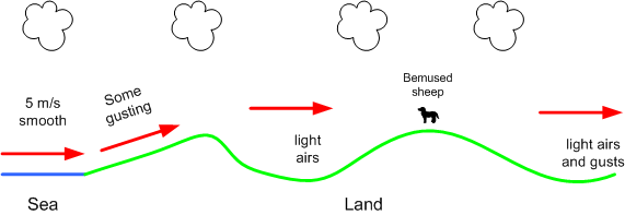
On 21-Sep-2013, I walked along a ridge from which there was a sea view, then dipped into a valley, as I walked along the path that lead to the next ridge I encountered a bemused sheep which continued to graze whilst I messed with a wind speed meter. Beyond this second ridge is an inland plain. On the seafront, the wind was blowing steadily at 5 m/s from the south west. The sketch below is an interpretation of the wind speed measurements I took along the way. On the slope up from the sea the wind blew steadily with some gusting as it did on the two ridge tops. In the valley, the air was still, with little movement in the tree tops. On the plain, there were some light gusts of wind. The red arrows suggest the path of the wind.
You can learn a lot about solar irradiance from one's own backyard, but studying the wind means leaving the house. From watching lost toy balloons, hot air balloons that I hope were not lost, walking and cycling around the town and countryside with a wind speed meter and looking at data from personal weather stations, I have formed the hypothesis that wind flows reasonably steadily of over hills and humps but is attenuated and gusty in the dips in between. If wind blows up a valley, there can be a funnelling effect in which case the valley ceases to be a place of shelter. In other words wind does not always flow parallel to the surface. As always, these comments should be treated with caution as other conclusions maybe possible with wider experience and greater knowledge.
On 21-Sep-2013, I walked along a ridge from which there was a sea view, then dipped into a valley, as I walked along the path that lead to the next ridge I encountered a bemused sheep which continued to graze whilst I messed with a wind speed meter. Beyond this second ridge is an inland plain. On the seafront, the wind was blowing steadily at 5 m/s from the south west. The sketch below is an interpretation of the wind speed measurements I took along the way. On the slope up from the sea the wind blew steadily with some gusting as it did on the two ridge tops. In the valley, the air was still, with little movement in the tree tops. On the plain, there were some light gusts of wind. The red arrows suggest the path of the wind.
I recently wrote a small programme to draw contour lines using SRTM data. Whilst this was written for some other purpose, I have used it to plot the terrain around a random selection of windmills (the sample size was 14) identified from Wikipedia. A little reading around the subject suggested that location of many mills is named "Mill Hill" (obvious with hindsight). If you Google "Mill Hill" you wind find a diverse list of places around the UK. Not all windmills are located on ridges and hills, but it is a favoured location. The graphic below shows a typical windmill location in a hilly region, the red contours are the high ground and the blue ones are the surrounding low lying area.
One source of wind data is aviation weather reports (Metars). It was whilst looking at the terrain on which airfields were located, it appeared that some which were laid out in the 1920's and 1930's are located on plateaus, like the one shown below. This observation is from a very small sample but may have some logic. A favourable wind would help getting a heavily laden and by today's standards, under powered aircraft off the ground
And my point is? The number of onshore locations where a wind turbine can be usefully be placed is constrained by terrain. This is further influenced by accessibility (almost everywhere belongs to someone) and acceptable land use.
Friday, 14 February 2014
Wind - Going off at a tangent
When I first became interested in the contribution wind and solar energy could make to a sustainable energy economy, a good starting point seemed to get an understanding of the energy available for conversion into heat or electricity. There is a lot of good wind data available in the public domain, so I started plotting out out wind speed distribution diagrams like to one below for a randomly selected group of worldwide locations.
I've had to put this work to one side for a few months, but not being the most disciplined of researchers, I wondered if the software used for the contour plots could be used to give an insight into the location of windmills. In reality, this was going off at a tangent, but the logic was that windmills are found in places for which there is no readily available source of wind speed data, thus studying their location would be an interesting way of looking at terrain and wind, this work has also been moved to one side, but I am looking forward to returning to it.
As is the way with these things, one question leads to several more. The first concerned the sample. Most "good" data is collected not amuse spreadsheet addicts, but to assist the safe passage of ships and aeroplanes which tend to operate from open, uncluttered spaces and often produce neat and tidy datasets which can be modelled with the Rayleigh or Weibull distribution (the Rayleigh distribution is a special case of the Weibull distribution in which the shape factor is constant at 2.0). Even without attracting attention to oneself by cycling around with a wind speed meter, it became clear that the wind speed distribution in places like backyards and some other parts of the urban and rural landscape where more complex.
Terrain is a factor in determining the amount of wind energy available at a given location. The average wind speed and distribution will be different at the floor of a valley from that at the ridges either side. These comments are drawn from work in progress from which as yet no definite conclusion as been drawn, thus they should be treated with caution. In general, offshore wind polewards of the tropics has a higher average speed than onshore and approximates to a Weibull distribution with a shape factor of 2.0. Onshore at a similar latitude, the average wind speed is lower than offshore and its distribution more skewed to the left, in terms of the Weibull distribution, the shape factor is often in the range 1.3 to 1.8, the higher values being associated with flat, open areas.
In an attempt to explore the effects of terrain on the distribution of wind speed, I plotted small contour maps using data from the SRTM mission, like the one shown below which is centred on a windmill close to where I live..
Terrain is a factor in determining the amount of wind energy available at a given location. The average wind speed and distribution will be different at the floor of a valley from that at the ridges either side. These comments are drawn from work in progress from which as yet no definite conclusion as been drawn, thus they should be treated with caution. In general, offshore wind polewards of the tropics has a higher average speed than onshore and approximates to a Weibull distribution with a shape factor of 2.0. Onshore at a similar latitude, the average wind speed is lower than offshore and its distribution more skewed to the left, in terms of the Weibull distribution, the shape factor is often in the range 1.3 to 1.8, the higher values being associated with flat, open areas.
In an attempt to explore the effects of terrain on the distribution of wind speed, I plotted small contour maps using data from the SRTM mission, like the one shown below which is centred on a windmill close to where I live..
I've had to put this work to one side for a few months, but not being the most disciplined of researchers, I wondered if the software used for the contour plots could be used to give an insight into the location of windmills. In reality, this was going off at a tangent, but the logic was that windmills are found in places for which there is no readily available source of wind speed data, thus studying their location would be an interesting way of looking at terrain and wind, this work has also been moved to one side, but I am looking forward to returning to it.
Wikipedia has some excellent lists of windmills from around the United Kingdom, and in may cases does the tedious task of converting National Grid coordinates to lat/lng relative to the WGS84 datum which are compatible with the SRTM data.
Windmills are part of the English landscape, especially in the eastern counties, but I was surprised at the number of them, maybe 2,000 (a guess) with the majority being built and operated in the 19th Century. At the beginning of the 20th century, the windmills were displaced by factories powered by steam, oil or electricity. For there to be so many windmills in operation, there must have been a substantial industry dedicated to their construction and maintenance together with a knowledge of the relationship between terrain an wind energy, I would be curious to know if there was a reference work on this?
In a week in which the UK has been lashed by some of the most violent storms in living memory, it should be remembered that the wind machinery has to survive under considerably harsher conditions than it normally operates. In storm conditions, wind turbines shut down in an attempt to minimize the risk of damage.
Windmills are part of the English landscape, especially in the eastern counties, but I was surprised at the number of them, maybe 2,000 (a guess) with the majority being built and operated in the 19th Century. At the beginning of the 20th century, the windmills were displaced by factories powered by steam, oil or electricity. For there to be so many windmills in operation, there must have been a substantial industry dedicated to their construction and maintenance together with a knowledge of the relationship between terrain an wind energy, I would be curious to know if there was a reference work on this?
In a week in which the UK has been lashed by some of the most violent storms in living memory, it should be remembered that the wind machinery has to survive under considerably harsher conditions than it normally operates. In storm conditions, wind turbines shut down in an attempt to minimize the risk of damage.
Labels:
economics,
Energy,
Renewables,
sustainability,
Wind
Friday, 17 January 2014
Diffuse Solar Iradiance
There are several models which can provide a good estimate of the solar radiation
received by a surface, one of the simplest is the Meinel model which relates
direct beam radiation to air mass. This formula is based on observations made
in the Mojave Desert in the 1960's. Whilst it does not take into account
atmospheric conditions such as water vapour and aerosols (minute particles
resulting from many human and natural processes) for which data is not always
readily available, it provides a reasonable estimate of direct bean, clear sky solar
radiation. The diffuse radiation is often estimated as a fraction of the direct
beam radiation, often a figure between 10 and 15% is quoted. However, it
became clear when looking at data from a variety of sources, that the diffuse
fraction increases as air mass increases. Clear sky diffuse irradiance is inversely proportional to air mass in
the same way that direct beam irradiance is, but the rate of decline is slower,
hence the increase in diffuse fraction.
This project is an attempt to produce a simple model for diffuse irradiance in southern England.
Comment
This is work in progress and has not be reviewed and should be treated with caution, It is an update on earlier one entitled "Then Diffuse Fraction" which has been deleted.
The Equipment
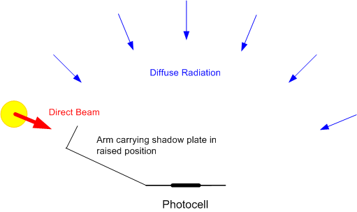
The equipment consists of a flat photocell mounted on a horizontal surface. This photocell has good cosine response. The short circuit current of the photocell is directly proportional to the irradiance, in this case the short circuit is provided by a 10 watt 1 ohm resistor, the voltage across indicates the current through the cell. An arm mounted in front of the cell carries a shadow plate. When this arm is raised, the photocell is in shadow and only receives diffuse radiation, when it is lowered, the photocell receives both diffuse and direct radiation. The concept is shown in the diagram below:
The device is constructed from Meccano and plywood. Three screws provide a means of obtaining a horizontal surface as indicated by a level gauge.The photo shows equipment in use.
Originally, the equipment was meant to be a prototype for something better,
however, as data has accumulated, I am reluctant to make changes and introduce
inconsistencies into the data. One useful enhancement would be to put an
amplifier into the circuit to increase the precision of the measurements which
is currently limited by capabilities of the multimeter.
Observations
Data is collected on days when a large part of the sky is clear, such days are rare in the south of England and accumulating a workable dataset is proving to be a slow process. Ideally, the analysis should be based on a full year's data, at the time of writing, there is only eight months from May 2013 to December 2013.
Observations have been made in a number of locations. For air mass values in the range 1.5 to 4.0 (mid morning to mid afternoon), the data appears to be similar for any open space, such as a public park ringed with trees. For higher values of air mass (around dawn and dusk), it is preferable to cycle to a south facing beach.
Dogs
One of the hazards of collecting data in public places is the attention of dogs, I like dogs, so this is not a problem, but it has resulted in some curious observations, for example, a freshly laundered poodle has a much greater effect on diffuse irradiance than a mud splattered labrador. This is thought to have no scientific interest.
General Comments
An important part of the data collection process is the notes taken at the time, these provided an explanation for some of the variance.
This project is an attempt to produce a simple model for diffuse irradiance in southern England.
Comment
This is work in progress and has not be reviewed and should be treated with caution, It is an update on earlier one entitled "Then Diffuse Fraction" which has been deleted.
The Equipment
The equipment consists of a flat photocell mounted on a horizontal surface. This photocell has good cosine response. The short circuit current of the photocell is directly proportional to the irradiance, in this case the short circuit is provided by a 10 watt 1 ohm resistor, the voltage across indicates the current through the cell. An arm mounted in front of the cell carries a shadow plate. When this arm is raised, the photocell is in shadow and only receives diffuse radiation, when it is lowered, the photocell receives both diffuse and direct radiation. The concept is shown in the diagram below:
The device is constructed from Meccano and plywood. Three screws provide a means of obtaining a horizontal surface as indicated by a level gauge.The photo shows equipment in use.
Observations
Data is collected on days when a large part of the sky is clear, such days are rare in the south of England and accumulating a workable dataset is proving to be a slow process. Ideally, the analysis should be based on a full year's data, at the time of writing, there is only eight months from May 2013 to December 2013.
Observations have been made in a number of locations. For air mass values in the range 1.5 to 4.0 (mid morning to mid afternoon), the data appears to be similar for any open space, such as a public park ringed with trees. For higher values of air mass (around dawn and dusk), it is preferable to cycle to a south facing beach.
Dogs
One of the hazards of collecting data in public places is the attention of dogs, I like dogs, so this is not a problem, but it has resulted in some curious observations, for example, a freshly laundered poodle has a much greater effect on diffuse irradiance than a mud splattered labrador. This is thought to have no scientific interest.
General Comments
An important part of the data collection process is the notes taken at the time, these provided an explanation for some of the variance.
- Haze. This was present on several summer days, the effect was to increase the diffuse irradiance to over 200 watts/m2.
- Low Level Cloud. If cumulus is forming or present in the sky, the diffuse irradiance will rise above the clear sky level. The presence of low level cloud implies that the relative humidity in the lower part of the atmosphere is close to 100%. In an otherwise clear sky, small fragments of cumulus can form and disperse very quickly. It seems that the formation of a cloud is preceded by an increase in diffuse irradiance.
- High Level Cloud. Except when the high level cloud is between the sun and the photocell, high level cloud causes little or no increase in the diffuse irradiance.
- Jet Trails. Occasionally, the total irradiance would dip as an airliner came between the Sun and the photocell. One morning, a larger than average jet trail appeared, this was probably created by an Airbus A380 bound for one of the Paris airports.
- Morning/Afternoon Variations. It is common for there to be significant differences in the irradiance before and after solar noon. In the south of England it is common for the sky to be clear during the first half of the morning after which clouds start to form, as a result, the irradiance is higher in the morning than the afternoon. In other climates, irradiance can be at a maximum in the early afternoon.
- Seasonal Variations. Two factors which influence solar irradiance are the water content of the atmosphere and aerosols and these vary according to the season and climate. In southern England the water content is higher in late summer and early autumn than in the winter months.
Calculations
In the South of England, the "economic" range of air mass is approximately 1.5 to 6.0. In this range the plane parallel method of calculating air mass provides a reasonable approximation and some computational convenience. The calculation (with the exception of the equation of time) is described on this page:
Sun-Earth Geometry
Results so far.
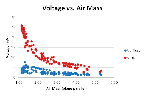
The first graph shows the voltages plotted against the plane parallel air mass:
Extracting the diffuse measurements and breaking them down by the state of the sky gives this graph:
The data for hazy days and those when there were a few cumulus in the sky are distinct from those when the sky was almost free from cloud or contained a few or scattered high level cloud such as cirrus.
First Attempt at a Model
Experience with this photocell suggests that its sensitivity is approximately 40 mA per watt/m2 as the resistor is 1 ohm, this becomes 40 mV per watt/m2. Discarding the haze and cumulus and amalgamating the clear and cirrus set and expressing the results as watts/m2 gives:
This is a reasonably tidy dataset, however data is not evenly distributed across the range of air mass, however, a simplistic curve fit using the same form of equation as the Meinell model has been attempted. It is probable that as more data is collected, the values of the constants will change.
At the time of writing, only limited testing has been done using this diffuse irradiance model. It appears that when combined with the Meinell model it produces better estimates of global horizontal irradiance than simply making the diffuse element a fixed fraction of the direct beam component. The graph below shows an estimate of the global horizontal irradiance for a clear, June day on the South cost of England, this appares to be reasonable when compared to the output of a personal weather station.
A more systematic evaluation will take place when a full year's data is available.
Correlations
For most locations, not much is known about the state of the sky at any given time. The nature of the irradiance can be source of information about the atmosphere. Initial attempts to correlate the data with derivatives of temperature and dew point data from the surface weather reports from the nearest airfield (approx. 7 km to the west) have not been successful. An initial attempt has been made to use data from NASA Aqua satellite obtained from the NASA Earth Observations website and this suggests an interesting line of enquiry.
If the data is broken down into three bands defined by aerosol optical depth, there is a suggestion that the data will segment:
Some of the highest values of V diffuse were observed when haze was clearly visible and haze is associated with high values of AOD, similarly, the lowest values were obtained when the AOD was also low. This is to be expected because AOD is one the inputs to parametric models of solar irradiance and it is also used as indicated of air quality.
A similar exercise with water vapour as less conclusive.
Variations on this theme using parameters based on surface temperature and dew point produced similar results.
Future Work
There are three tasks:
In the South of England, the "economic" range of air mass is approximately 1.5 to 6.0. In this range the plane parallel method of calculating air mass provides a reasonable approximation and some computational convenience. The calculation (with the exception of the equation of time) is described on this page:
Sun-Earth Geometry
Results so far.
The first graph shows the voltages plotted against the plane parallel air mass:
Extracting the diffuse measurements and breaking them down by the state of the sky gives this graph:
The data for hazy days and those when there were a few cumulus in the sky are distinct from those when the sky was almost free from cloud or contained a few or scattered high level cloud such as cirrus.
First Attempt at a Model
Experience with this photocell suggests that its sensitivity is approximately 40 mA per watt/m2 as the resistor is 1 ohm, this becomes 40 mV per watt/m2. Discarding the haze and cumulus and amalgamating the clear and cirrus set and expressing the results as watts/m2 gives:
This is a reasonably tidy dataset, however data is not evenly distributed across the range of air mass, however, a simplistic curve fit using the same form of equation as the Meinell model has been attempted. It is probable that as more data is collected, the values of the constants will change.
At the time of writing, only limited testing has been done using this diffuse irradiance model. It appears that when combined with the Meinell model it produces better estimates of global horizontal irradiance than simply making the diffuse element a fixed fraction of the direct beam component. The graph below shows an estimate of the global horizontal irradiance for a clear, June day on the South cost of England, this appares to be reasonable when compared to the output of a personal weather station.
A more systematic evaluation will take place when a full year's data is available.
Correlations
For most locations, not much is known about the state of the sky at any given time. The nature of the irradiance can be source of information about the atmosphere. Initial attempts to correlate the data with derivatives of temperature and dew point data from the surface weather reports from the nearest airfield (approx. 7 km to the west) have not been successful. An initial attempt has been made to use data from NASA Aqua satellite obtained from the NASA Earth Observations website and this suggests an interesting line of enquiry.
If the data is broken down into three bands defined by aerosol optical depth, there is a suggestion that the data will segment:
Some of the highest values of V diffuse were observed when haze was clearly visible and haze is associated with high values of AOD, similarly, the lowest values were obtained when the AOD was also low. This is to be expected because AOD is one the inputs to parametric models of solar irradiance and it is also used as indicated of air quality.
A similar exercise with water vapour as less conclusive.
Variations on this theme using parameters based on surface temperature and dew point produced similar results.
Future Work
There are three tasks:
- Continue collecting data when the opportunity arises until at least until April 2014 to obtain a dataset extending over a full year.
- Determine if the same process can be extended to create a location specific model for direct normal irradiance. This can be calculated from measurements of global and diffuse horizontal irradiance, however, the equipment in its present form may not be able to provide data of adequate quality without modification.
- Attempt a model which accounts for seasonal variation.
Acknowledgement and Appreciation
Data relating to Aerosol Optical Depth and Water Vapour was obtained from the NASA Earth Observations website. The data available on that site is highly instructive and I would like to express my appreciation to NASA and NOAA for making it available.
Friday, 3 January 2014
Starting over
Not too far from where I live is a house that was built sometime in the 1980s, I guess it was none too comfortable to live in. Whilst it was being partially demolished, I did not see any signs of insulation, just a lot of windows with rotting frames and a load of rusting radiators. Technically, it is being extended, but in reality, it is being rebuilt. The roof is well insulated, the walls have a 100 mm layer of polystyrene and the windows are double glazed. Not wanting to be a nosey neighbour, I have not enquired about the heating system, however, I know that a wood burning stove was installed in a similar development and has yet to be lit. Retrofitting a property to that standard would be difficult and expensive and unlikely to pay-back. That statement is based on a study of my own home where you could spend a lot of money, not be much warmer and would lose the character of an airy Edwardian semi.
Sustainability is much easier to attain with a clean start. I am currently working on (more accurately "staring at") an electrical storage project. Storage is one of the key components in a sustainable energy economy, but batteries are DC devices and my home is wired for AC. AC is a logical choice for distributing electricity, but increasingly it is consumed at DC. Some time back I did a quick survey on how we use electricity in our home and produced this graph, this suggested that only 15% of electricity has to be consumed at 240 volts/AC or in other words the washing machine and vacuum cleaner. Some things like the fridge are available in low voltage DC forms, computing and entertainment devices all have power supplies to shift from high voltage AC to low voltage DC. We are slowly migrating the lighting from CFL to LED devices. Each LED light bulb has its own power supply circuit for AC to DC conversion.
Even though most things use low voltage DC, distribution within the house is 240 volts AC, That was a logical way of doing things in the 1920s when electricity was first installed and all appliances used AC, the better part of a century later, there may be some value in examining household distribution.
If storage were to be part of the household energy system without any radical changes in wiring, the first step would be go from 240 volts AC to 12 or 24 volts DC for battery charging, the battery would be connected to an inverter to get back to 240 volts AC to go through the ring mains, devices connected to these would then drop it back to low voltage DC. This would be a complex and inefficient system and one which is not going to get built any time soon. The small DC storage project is all DC, albeit with some level shifting, and is relatively simple.
I stumbled over another example of the complexity of legacy systems. When the railways moved from steam engines to electric motors, high voltage DC was chosen because at the time only DC motors could provide the high starting torque needed to get a train moving. Modern electric trains (so I am told) use AC motors. Thus the grid feeds trackside substations with AC, this is converted to DC for the trackside rails, the train then converts it back to AC. I doubt if the losses in this system are great, but the result is a complex system with DC for traction and 3 phase AC for everything else.
In the UK there is a debate over how to curb emissions which can be grossly oversimplified to nuclear versus the renewable technologies such as wind and solar. My own view is that there should be different paths for "old" systems and "new" developments. For the legacy systems which are based on large amounts of uninterrupted energy from fossil/nuclear sources, the key technologies are conservation and energy management. It is valid to determine if it is possible, practical and economic to build new systems which are more or less dependent on renewable resources which are discontinuous (the Sun does not shine at night and the wind does not always blow), these would incorporate appropriate technologies, e.g. LED lighting and storage. It's so much easier to design these things from scratch and not have to mess with the past.
Labels:
Conservation,
economics,
Energy,
History,
LED,
Renewables,
Solar.,
sustainability,
Wind
Subscribe to:
Posts (Atom)